https://jetbrains.github.io/mps-coderules
Revision: 0.9.0
Date: 27 May, 2021
About Coderules
Type inference and type checking is a problematic area for language authors — users of JetBrains MPS, because of inherent intricacies of the problem itself and sometimes less than adequate support from the framework.
CodeRules is a new technology that brings logic programming in the form of constraints processing as a vehicle for implementing type inference.
Typesystem in MPS is traditionally defined with help of type checking rules, in particular inference rules, which allow for making logical statements about types, such as “is a” or “is a subtype of”, enabling the internal engine to infer the specific type, deriving it from a collection of such statements, which are referred to as type equations and inequalities.
(statement in j.m.lang.typesystem language)
Albeit brief and concise, this notation leaves many questions unanswered when it comes to how exactly the system of equations and inequalities is processed. In other words, type inference is — for the most part — left up to the internal engine to decide.
This limits the options for the author of typesystem to control how exactly subtyping is defined, and what happens with type parameters when computing sub- or supertype. Java, for instance, has several kinds of “conversions” with clearly defined rules controlling how types are transformed and what types are compatible in certain situations. All of this has to be emulated with “strong” and “weak” subtyping in MPS.
Consider how type of a method call is calculated: details aside, in essence when_concrete has to be applied to types of each argument. Then we should either turn to inequalities and rely on the inference engine, or analyse the type structure and run closing computation when the last unknown type is finalised.
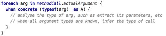
(example of processing method arguments)
Coderules may have a solution to these and other issues. The core idea is to employ a constraints processing system to process facts and relations, collectively known as constraints, with the user being in full control of what constraint rules to generate for given source model. With logical variables representing unknowns, and with support for pattern matching making use of term algebra and unification, it should be straightforward to define the core of type inference or a similar framework without having to rely on opaque implementation and pre-defined relations.
To illustrate the idea, let’s look at a couple of examples. These are taken from the typesystem implementation for BaseLanguage.
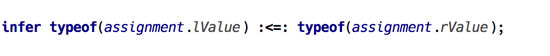
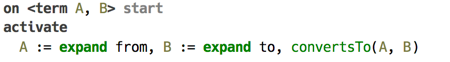
Type checking assignment expression could look like the following. What the code says is basically: once left and right sides of the assignment have types (not necessarily ground types), test if left side’s type converts to right side’s. Constraint convertsTo/2 is defined in the same aspect, and the typesystem author has full control how it deals with type parameters, for example.
(type checking assignment with constraint rules)
Instead of waiting until a type has been finalised in order to access its structure, pattern matching is used to trigger constraint rules only on types of certain form. The example below shows how convertsTo/2 is resolved for an instance of LowerBoundType.
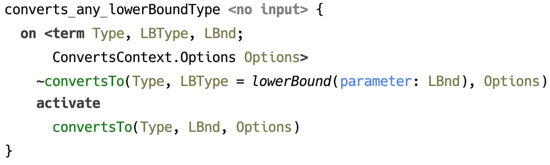
(resolution of convertsTo/2 constraint using pattern matching)
Features
-
A language for constructing rule templates that are applied to source model and may include constraint rules. The rules may be concept-specific or standalone.
-
Constraint Processing System — an extension of CHR1 semantics allowing the use of unification in a constraint rule’s head with automatic binding of logical variables on successful match. This extension also supports alternative body branches, as well as calling arbitrary Java code.
-
A framework for executing a constraint rules program, with support for error reporting from rules’s body. The UI also includes a tracing tool for providing insights into how constraints are processed.
Examples are provided that demonstrate the use of this technology for type checking.
Table of contents
This documentation site is organized as follows:
- CodeRules Language discusses the language features
- Evaluating CodeRules Program explains the internals of CodeRules
- Examples include the following:
- All documentation on single page
Contacts
The project is hosted on GitHub, latest builds can be found here.
The author can be reached by email fedor.isakov@jetbrains.com or on Twitter.
JetBrains MPS is a project developed by JetBrains and is available via web and Twitter
Copyright
All contents is copyright © JetBrains 2021. All rights reserved.
-
Constraint Handling Rules http://www.informatik.uni-ulm.de/pm/fileadmin/pm/home/fruehwirth/constraint-handling-rules-book.html ↩
CodeRules Language
The language jetbrains.mps.lang.coderules defines the core concepts listed below.
Constraint rules
Constraint rules are the basic constructs that enable the use of logic programming with constraints and predicates combined into logical clauses.
Rule templates
Defined in a rule table root, these are the fundamental building blocks of CodeRules program. These are either static or concept-specific rules that get applied to appropriate nodes in the source model and are able to use the constraint rules to implement their logic.
Macros
Macros extend the expressiveness of constraint rules with the ability to refactor away fragments of a rule’s body. Macros are provided by macro table.
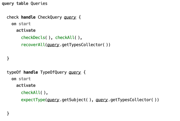
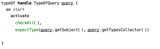
Queries
With help of queries one builds integration of CodeRules into the language aspect. Typechecking aspect provides query kinds that correspond to actual use cases implemented by type checker.
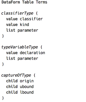
Terms
One important feature of CodeRules is the ability to abstract away from type structure defined by the language. For example, one may decide to represent all primitive types of BaseLanguage as a term primitive(kind=<specific kind>).
Term table contains declarations of terms which are used as internal representation of types.
Lists
Language Aspect
Coderules are defined in tables, which are root concepts of language jetbrains.mps.lang.coderules. Rule tables and other related roots should be created in a language’s aspect model corresponding to the specific kind of analysis performed. The language jetbrains.mps.lang.typechecking declares the aspect types.
Root concepts
The following table contains root concepts that belong to CodeRules language structure.
| Concept | Description |
|---|---|
| Rule Table | contains rules and constraint declarations |
| Term Table | defines terms, the data structure that is used in unification |
| Macro Table | facilitates the reuse of body template fragments |
| Query Table | collection of entry points to the constraints program |
Constraint Rules
At the core of CodeRules program lies the concept of constraint rules, which captures the essence of logical programming. The structure of a constraint rule enables to express a program as a list of logical clauses, each consisting of the head — the list of antecedents, and the body — the list of consequences. Both the head and the body are represented as lists of constraints and predicates. More on the semantics of constraint rules can be found in the section on constraints processing.
(example of a constraint rule in a rule template)
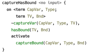
A constraint rule can be created at any place within a rule template’s body with the help of a keyword on. A constraint rule within a loop generates a runtime constraint rule on every iteration of this loop.
A constraint rule must include either a body or a head, no constraint rule can omit both.
Head
Constraints in a constraint rule’s head can be declared as either kept or replaced. Replaced constraints are marked with a tilde ~.
There is a certain limitation as to what constraints can be used in rule’s head: it can only contain constraints defined by this rule table, or one of the rule tables it extends.1
A constraint rule with an empty head, not declaring any constraints to serve as its input, is considered an automatic rule and is triggered automatically on start of constraint rules program execution.
Guard
The guard is optional and may contain only predicates or the $() expression which evaluates boolean-typed Java expression.
Predicates, also known otherwise as “built-in constraints” are represented either as binary operators, such as = for unification or == for equality, or they are boolean-valued functions. Unification or equality if used in guard, only tests that its arguments can be unified, otherwise if called from body, it invokes the actual unification or assigns the value to a logical variable.
There are also predicates that can only be queried, such as isFree/1 or isAssigned/1, testing if a logical variable is free or has value assigned. Such predicates can only be used in guard.
(example of predicates used in guard)
Body
Constraint rule’s body can contain any visible constraints declared by rule tables located in imported models, as well as predicates.
(unifies predicate used in the guard and in the body)
A body may contain two or more alternative branches, which essentialy capture the idea of evaluating constraint rules with backtracking. Namely, the evaluation starts with the first branch, and in case it is finished without failures, other branches are not evaluated. On failure the second branch is evaluated, etc.
(example of a constraint rule with alternative branches)
A body may be created with the help of a template fragment — a block of code that produces constraints and macro calls via special emit statements: <%…%>.
(example of constraint rule with a body template)
Logical variables
A constraint rule can declare logical variables. By default a logical variable ranges over terms, although any Java object may serve as a value. A logical variable is used whenever a term or a term feature needs to be represented in a logical clause.
(constraint rule declaring logical variables)
When a constraint with logical variable as one of its arguments is matched, that variable becomes bound to the corresponding argument of the matching occurrence. The scope of such binding is this constraint rule’s guard and the body.
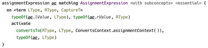
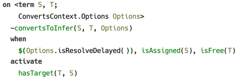
To illustrate how automatic binding of logical variables work, consider the following example. Constraint typeOf/2 associates a type with a location in source model, and constraint convertsTo/2 ensures its 1st argument can be converted to the 2nd, which must both be terms.
(example of binding the logical variables)
This constraint rule is triggered when both locations referred to as ae.lValue and ae.rValue have their types assigned, as both typeOf/2 constraints must be present for a match to be successful. Once a constraint rule’s head is matched, both logical variables LType and RType become bound to whatever was the 2nd argument of corresponding typeOf/2 constraint.
It’s important to note, that although on successful match both lValue and rValue have types, it’s not guaranteed that these types are ground. A type may be represented by a free logical variable, or a term containing free variables.
Another very important thing to notice is that a logical variable enjoys full privileges of being an argument to a constraint. Which means, if in the above example both variables are free, and LType = RType, then both locations will have essentially the same type (in the sense of “same instance”), not just matching types.
Pattern matching
There is support for pattern matching, using terms as patterns, which may optionally contain logical variables. For this to work, a logical variable that serves as a constraint argument should have a pattern attached.
The following example illustrates the use of pattern matching in a constraint rule’s head. Here, the first argument to constraint convertsTo/2 in the head is a logical variable with pattern expression. In this case the constraint rule will only be triggered if the active constraint’s first argument is bound (is not a free logical variable), and it matches the pattern.
(constraint rule with pattern matching)
Evaluation of Java expressions
Arbitrary Java code can be called with $() predicate. It accepts either an expression of boolean type, in which case it can be used in guard, or expression of any type when called from body. In the latter case, the value expression evaluates is ignored.

(example of using $() predicate)
Using macros
In order to make use of macro definitions, which are essentially parameterised templates extracted to a separate root, one of the two pseudo predicates can be used: expand and call. The former accepts a node, whereas the second expects the arguments that are substituted as macro parameters.
-
This limitation has its origin in the way constraint rules are chosen when an active constraint is being processed. Namely, constraint rules to match an active constraint are selected from the rule table declaring this constraint, and rule tables that are its extensions. The order of constraint rules within the rule table matters, the ones declared on top are matched first. Productions from extending rule tables are prepended to the list of constraint rules of the rule table they extend. ↩
Rule Table
Constraint declarations
Constraints declared by a rule table are public symbols that serve as its API in the following sense. In the head of constraint rules of a rule table and its extensions, only those constraints can be used that were declared in this rule table or any rule table it extends. On the other hand, any constraints can be used in body, provided the references to constraint declarations are resolved in the usual way.
Rule templates
Rule templates defined in rule tables are responsible for implementing the logic of checking the types (or other kind of code analysis), for which they may contribute constraint rules. These are created with a DSL that allows mixing constraints and Java code, and can also include constraint fragments inside a constraint rule template.
A rule table is a concept in language jetbrains.mps.lang.coderules.
(example of a rule table declaration — without contents)
Keyword extends allows to specify another rule table that is to be extended. All constraint rules generated by templates in this rule table will have higher priority. This enables to override the original rule table’s behaviour.
The following example demonstrates how a constraint rule’s body is constructed using a template. A body template is enclosed into a pair of %% … %% symbols and yields constraints wrapped into special <% … %> brackets.
(example of constraint rule with body template)
As demonstrated above, a constraint rule can be created depending on the result of evaluating a condition expression. Constraint rules can also be created in a cycle.
Only declared constraints are allowed to be used in the heads of constraint rules in the rule table declaring the constraint or the extensions of this rule table. Rule table should declare one or more constraints, unless it only uses the constraints from rule tables which it extends. Constraint declaration consists of name and arity, which together constitute a constraint symbol. Constraint’s arity is fixed.
Rule templates can specify applicable concept, either exactly or including its subconcepts. One can also declare standalone rules, which are applied automatically on every evaluation of CodeRules program.
(example of standalone rule without input)
Rule template’s contents is a block of code that gets executed when the rule is applied to the source model. If the input is specified, the declared parameter is available in rule’s body.
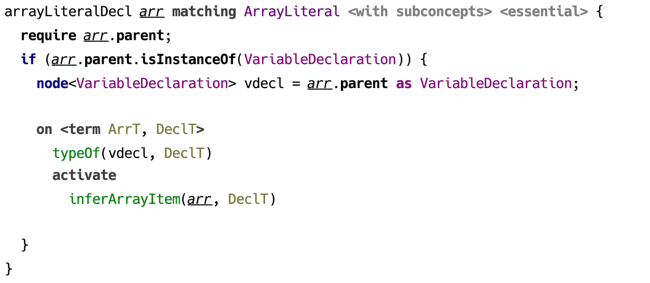
Rules may affect the scope of model locations that are processed during an evaluation session. Suppose a constraint rule responsible for type checking a particular location in source model relies on presence of constraint rules that are only available if some other location is processed as well. To guarantee that a certain model location is processed during the evaluation session, one uses require statement.
(example of using require statement)
This feature comes in handy for implementing a “partial” type checking (a.k.a. “local type checking”). Type checking may be launched either for a whole root, processing all AST tree recursively, in which case it may be called a “total” type checking, or it can be launched for a particular AST node in isolation, and this is then a “partial” type checking. In the latter case, there must be additional information provided by the typesystem author, which should serve to establish the necessary context by means of following the required dependencies. These may be method and class declarations, for example, if we are to check the type of a particular method parameter.
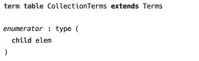
Term table
Term table contains term declarations. A term is a simple recursive data type that is suitable for implementing unification. Also, terms can model any other data structure, in particular they are suitable for representing types in a programming language.
A term is defined by its symbol and its features, which can be a child term, a list of children terms or any Java object1.
(example of a term declaration)
An open term declaration can be extended by another term, which helps implement a structural subtyping on terms. A term extending another term can add new features.
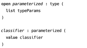
(example of open term declaration)
A instance of classifier() can always be matched with a pattern parameterized(), because the former structurally extends the latter.
A term table can extend another term table, in order to provide extensions to existing terms.
(example of a term table extension)
-
Java object conforming to equals/hashCode contract ↩
Macro table
The motivation behind using macros, and — in a wider context — behind using terms as datatype, is that sometimes it takes more than just an SNode to represent a type. For example, in order to find a solution for a type inference problem, a logical variable representing the inference variable requires a bound, implemented is a constraint on that variable. In other situations, a newly constructed type has to substitute type variables with some other types. It is only convenient to extract such functionality into a separate, reusable fragment.
The two kinds of macros — expand and call — are provided to refactor portions of constraint rule templates by introducing reusable fragments. Both kinds of macros are only available in body part of constraint rule templates.
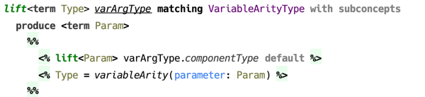
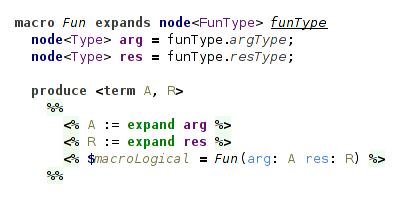
Expand macro
Expand macro has access to SNode instance on which it was invoked, can access the optional parameters, and either use or assign the logical variables. By contrast with rules, expand macros are always explicitly invoked.
Expand macro declaration must define the applicable concept. It may also contain one or several parameters, which are optionally provided at the usage site and are made available to instances of the macro.

(example of an expand macro declaration)
Logical variables declared in angle brackets right after the name of the macro are used to pass IN and OUT parameters. In addition, a macro can define its own logical variables.
A specific expand macro is always applicable to SNode instances of particular concept that must extend the concept in the macro declaration, which it refers.
Expand macro can be applied recursively to provide more fine-grained reusability.
(example of a recursive expand macro)
Substitution — passing parameters via context
Call macro
A call macro can be most simply described as a method accepting one or several parameters and a list of logical variables. A call macro can be invoked from a constraint rule’s body, as well as from an expand macro or another call macro.
(example of a call macro declaration)
Macro table extensibility
A macro table is able to extend other macro table in order to provide definitions of expand macros.
(example of a macro table that extends another macro table)
Query table
Query is the entry point to a CodeRules program. The only purpose of a query is to activate constraints that trigger computations necessary for the query logic. Essentially a query is a limited constraint rule that only has the body part.
(example of a query)
A query is discovered by the API through its kind, which is specific to the language aspect, and which is represented as a Java interface. Query declares its kind in the handle section. The body of a query can contain same constraints and predicates as regular constraint rules.
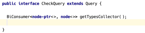
(example of a query interface)
Evaluating CodeRules
Analysis of source model with CodeRules can be described as a two-phase process.
- Collecting rule tables and applying rule templates.
- Processing constraint rules collected in the first stage.
In the first phase, languages used by the model being analysed and surveyed for the appropriate CodeRules aspect model, which is types in case of type checking.
The outcome of this phase is a constraint rules program, which is a collection of rule tables, which in turn represent lists of constraint rules. This “program” however, exists in memory only as it does not have any textual representation.
In the second phase the constraints program that was created in phase one is evaluated. Evaluation starts with a query, which serves as an entry point to the program.
Queries correspond to usual procedures that analyse the source mode, such as typeOf or convertsTo, and are declared in the same aspect model.
(example of a query)
Applying rule templates
The first stage of evaluating CodeRules program begins with collecting rule tables. Rule tables are collected from corresponding aspects of all languages imported into the model. In addition to that, all extended languages are also included into the scope.
All rule tables collected in the previous step are sorted, so that the ones coming from extensions appear earlier. This sorting order ensures that when constraint rules are selected to match an active constraint, the constraint rules coming from extensions will have higher priority.
After the relevant rule tables are collected, the source model is traversed from the specified location, and the applicable rules are evaluated. As rule templates are applied, they produce constraint rules. As well as generating constraint rules, the rule templates are allowed to report messages to be displayed at source locations.
Generated constraint rules constitute the constraints program, which is then executed in the next stage.
Executing constraints program
In the second stage the constraints program is executed.
To begin execution, a query is selected, which contains the list of constraints to be activated. Query can be viewed as a regular constraint rule, which is triggered unconditionally.
There is a fixed order in which constraint rules are fired on start of program execution. First, all “on start” constraint rules are triggered. All constraints activated by these constraint rules are processed normally, and after there are no more constraint rules to be triggered, the query is fired.
Order of constraint rules fired:
- “on start” rules
- query
While constraints program is run, it is allowed to report feedback, such as assign calculated types or report problems, using special constructs, that are available as predicates in the body of a constraint rule.
Failures may be encountered during constraints program execution, such as a unification failure, and they are caught with the help of alternative body branches, when those are provided. An uncaught failure terminates program execution and is reported to the user.
In the following example, a potential error is caught in the else branch and a corresponding errors is reported. Execution of constraints program is not terminated though, so other problems may still be reported.
(example of using an alternative body branch)
User interface
The user interface is defined by a plugin responsible for particular language aspect.

(context menu with type checking actions)
Activation trace view
During execution of a constraints program all activation/suspension/deactivation events, as well as ask/tell queries to predicates can be displayed in a dedicated view.
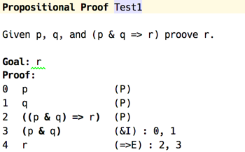
(sample proof in propositional logic)
Above is an example of a proof in propositional logic, the trace of checking which is provided below. The rows in the left pane correspond to events happening during constraints processing, such a constraint activated or suspended, or a constraint rule triggered. When a row in the left pane side selected, the right pane displays the contents of constraints store captured at the moment the event occurred.
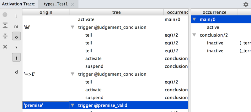
(activation trace view)
Constraints Processing System
This section briefly overviews how constraints processing works. The system described here follows loosely the CHR specification, and has been in particular heavily influenced by JCHR1 implementation. The distinctive features are built-in support for logical variables, terms, and pattern matching. Alternative body branches are a deviation from the standard CHR.
Terms and unification
Constraints processing relies heavily on the use of terms as data type. Abstractly speaking, terms are functions of zero or more arguments. Any opaque value captured by a term must be a POJO.
  f(g(), h(k()))

  p(val("foo"), q())

  node(name("List"), arg(node(name("Int"), arg())))
(examples of terms)
The unique feature of terms is that they support unification. Unification of two terms is possible with or without variables being used as subterms of either participant, but in the latter case the two terms must be equal.
A term variable ranges over terms. A substitution is a mapping of variables to terms. Unification searches for a substitution $\sigma$, such that for two terms being unified, $f$ and $g$, the following holds: $\sigma f = \sigma g$. For example:
  [X -> g()] unifies f(X, h(X)) and f(g(), h(g()))

  [X -> Z, Y -> g(X)] unifies f(X, g(X)) and f(Z, Y)
The latter unifier is the most general one, since other substitutions that also unify the two terms are all subsumed by it:
  [X -> g(X), Y -> g(g(X)), Z -> g(X)]
  [X -> g(g(X)), Y -> g(g(g(X))), Z -> g(g(X))]
Unification may fail because the arity or the symbols of the two terms mismatch. Also, since infinite terms are not supported, unification may fail because of occurs check, which means a variable can’t be unified with a term, that itself or through its descendants has this variable as one of its arguments.
  f(X, h(X)) and f(g(), h(k())) can't be unified because g != k
  f(X, g(X)) and f(g(X), g(h()) can't be unified because of
                                failed occurs check
Pattern matching is possible when variables are only used by one of the terms, which then serves as a pattern. To test if a pattern matches a given term can be implemented by a linear time algorithm, whereas full unification is slightly more complicated.
Logical variables
Logical variables serve to identify an object that is to be determined in the future. They are monotonic, in the sense that once a variable is assigned a particular value, it stays assigned to that value. In addition, they implement a union-find data structure2 a.k.a. “disjoint set”. Any free logical variable can be assigned a class by setting its “parent” field to point to the class’s representative. All logical variables belonging to the same class are treated as exactly one variable. Logical variables notify observers when they become ground and when their parent (class representative) changes.
  val X = Logical("X")
  val Y = Logical("Y")

  assertTrue(X.isFree() && y.isFree())

  X.set("foo")
  assertTrue(X.value() == "foo"))

  Y.union(X)

  assertTrue(Y.find() == X)
  assertTrue(Y.find().value() == "foo")
(example of using logical variables)
A term variable can also be a logical variable, so that when two terms are unified, the substitution already has the calculated value for that variable.
  val X = Logical("X")
  val t1 = term("f", var(X), term("g", var(X)))
  val t2 = term("f", term("h"), term("g", term("h")))

  assertTrue(X.isFree())

  val substitution = t1.unify(t2)

  assertTrue(substitution.isValid())
  assertTrue(X.find().value() == term("h"))
Constraints and predicates
Constraints are, simply put, tuples with fixed arity and a symbol attached. In some respects constraints correspond to rows in a database table. Logically they can be understood as facts, relations, or propositions. An argument to a constraint can be a term, a logical variable, or any POJO, except another constraint.
Constraints are activated from a constraint rule’s body and stay active until there are no possible matches with any of constraint rule’s heads. If a constraint is not discarded by a constraint rule, it is stored for future use. Stored constraints represent the program’s state.
The following figure shows the lifecycle of a constraint. The big rounded square in the middle contains the states, in which a constraint is considered “alive”: it can be either “active” or “stored”, but available for filling up vacant positions in a constraint rule’s head. A stored constraint can be reactivated if one of its arguments changes, such as when a logical variable becomes ground.
A successfully fired constraint rule, which declares one or more of constraints in its head to be “replaced”, causes these to be terminated.

(lifecycle of a constraint)
Predicates
Whereas a constraint serves to embody a fact or a relation among objects simply by being a witness of such a fact or a relation, a predicate3 helps to establish a fact or a relation, or check if one exists, by means of executing a procedure. Same is true for facts and propositions.
Predicates must implement ask/tell protocol. If a predicate is invoked from constraint rule’s guard clause, it represents a query (ask), and if it is invoked from the body, it is an assertion (tell).
Example of a predicate
Example of ask/tell
Example of failed predicate
Constraint rules
Constraints program is built from constraint rules. Each rule has three parts: the part that is responsible for triggering the constraint rule, called “head”, the part that checks for pre-conditions, called “guard”, and the part that is evaluated when constraint rule is fired, which is called “body”.
Head
Head is a set of constraints which are all required to be alive in order for a constraint rule to fire. This set is divided into “kept” part and “replaced” part, the latter containing constraints that are to be discarded as soon as the constraint rule fires.
A constraint rule is triggered when there are constraint occurrences matching all constraints specified in constraint rule’s head. These occurrences include the active constraint, plus any additional matching constraints that are currently alive, filling the other vacant slots.
There is some terminology inherited from CHR that can be useful when discussing the kinds of constraint rules. In the following table E and E' are the set of constraints in constraint rule’s head, C is a conjunction of predicates serving as guard, and G is a conjunction of predicates and constraints in constraint rule’s body.
“kept” set E |
“replaced” set E’ |
Notation | Designation |
|---|---|---|---|
| empty | non-empty | E’ <=> C | G |
Simplification |
| non-empty | empty | E => C | G |
Propagation |
| non-empty | non-empty | E \ E’ <=> C | G |
Simpagation |
Essentially, a constraint rule with only “kept” constraints in its head is a “propagation”, the one with only “replaced” constraints is a “simplification”, and the one that has both “kept” and “replaced” constraints is a combination of the two.
In addition, we define a fourth kind of constraint rule, an “auto” constraint rule with an empty head. As the name implies, such constraint rule is triggered automatically on start of constraints program execution.
Guard
Guard is a conjunction of predicates, which are checked before a constraint rule is fired. Predicates in a guard are queried.
Body
Body is a conjunction of predicates and constraint activations. When triggered, each body clause is evaluated in order, with predicates serving as assertions and constraint activations producing new constraints. Each newly activated constraint is checked against any constraint rules that can be fired, and so on.
Triggering a constraint rule
The procedure processActive() accepts a constraint occurrence that has been activated and proceeds as follows until this constraint is either discarded or suspended (moved to store). This procedure calls itself recursively on every constraint activation, so there might be many active constraints at any given moment, organised into a stack, which matches exactly the call stack of processActive().
First, the procedure searches for “relevant” constraint rules that declare a constraint in their heads matching the active constraint occurrence currently being processed. These constraint rules form a FIFO queue, corresponding to the order of constraint rules within a rule table.
For each “relevant” constraint rule, which at least partially matches the currently active constraint occurrence, the vacant slots in constraint rule’s head are filled with matching constraints from the store, which were previously suspended. Once a full match with constraint rule’s head is established, the guard is checked.
A constraint rule together with a set of constraints matching the ones declared by its head, one of which must be the active constraint, is considered to have been triggered after the guard check returns true. Otherwise this constraint rule is skipped.
After a constraint rule is triggered, first the constraints marked by constraint rule’s head as replaced are deactivated, and the logical variables defined by patterns are assigned appropriate values by asserting equality through equals predicate. Then the constraints and predicates defined in constraint rule’s body are activated one-by-one. Every activation of a constraint is a recursive call to processActive().
If after having processed all items in constraint rule’s body the constraint occurrence currently being processed is still “alive”, meaning it has not being discarded during one of the recursive calls to this procedure, the process of matching and triggering constraint rules continues with the next constraint rule from the queue.
When there are no more constraint rules that can be matched, or the active constraint has been discarded, the procedure processActive() finishes. If, when the procedure is finished the active constraint is still “alive”, it is suspended and moved to the store.
Alternative body
Example of executing a program
Consider the following example of the Euclid algorithm taken from the CHR book4:
gcd(0) <=> true
gcd(N) \ gcd(M) <=> 0 < N, N =< M | gcd(M - N)
To illustrate the idea of using stored constraints to fill vacant slots when matching a constraint rule, let’s see what happens when this program is evaluated with 4 and 6 as arguments to gcd/1 constraint.
| Constraints store | Active constraint | Match | Result |
|---|---|---|---|
{} |
gcd(4) |
no constraint rules matched | suspend gcd(4) |
On activating gcd(4) there are no matching constraint rules, so the constraint is suspended.
| Constraints store | Active constraint | Match | Result |
|---|---|---|---|
{gcd(4)} |
gcd(6) |
gcd(6) \ gcd(4) |
guard condition fails |
{gcd(4)} |
gcd(6) |
gcd(4) \ gcd(6) |
discard gcd(6), activate gcd(2) |
Notice how both combinations of gcd(4) and gcd(6) constraints are tested. In general, if there are $n$ usages of constraint foo in a given constraint rule’s head, there will be $n!$ potential matches to be evaluated, so that all permutations are covered.
The last activation above is a recursive call to processActive(), so the cycle repeats. The active constraint has been deactivated, but contents of the store is unchanged.
| Constraints store | Active constraint | Match | Result |
|---|---|---|---|
{gcd(4)} |
gcd(2) |
gcd(2) \ gcd(4) |
discard gcd(4), activate gcd(0) |
{} |
gcd(0) |
gcd(0) |
discard gcd(0) |
There are no more constraint rules to match for gcd(2) as the active constraint, so it is suspended. But the constraint gcd(6) has been already discarded, so there are no more active constraints and the process stops. Here is the full trace of this program execution.
| Constraints store | Active constraint | Match | Result |
|---|---|---|---|
{} |
gcd(4) |
no constraint rules matched | suspend gcd(4) |
{gcd(4)} |
gcd(6) |
gcd(6) \ gcd(4) |
guard condition fails |
{gcd(4)} |
gcd(6) |
gcd(4) \ gcd(6) |
discard gcd(6), activate gcd(2) |
{gcd(4)} |
gcd(2) |
gcd(2) \ gcd(4) |
discard gcd(4), activate gcd(0) |
{} |
gcd(0) |
gcd(0) |
discard gcd(0) |
{} |
gcd(2) |
no constraint rules matched | suspend gcd(2) |
After the program has finished, the constraint store consists of only one constraint gcd(2), which is the GCD of 4 and 6.
Semantics of a constraint rules program
The paper by Betz and Frühwirth5 gives an excellent treatise on semantics of CHR using linear logic. Since this constraints processing system is based on CHR, this semantics is valid for it also.
Linear logic abandons boolean values and replaces them with consumable resources. Consequently, it introduces its own set of connectives, from which we are interested only in the following: $!,\otimes,\multimap$. The multiplicative conjunction $\otimes$ combines two or more resources that are all available at the same time. The symbol $!$ (of course) marks a resource that can’t be exhausted. And instead of implication $\rightarrow$ one uses $\multimap$ symbol, the meaning of which is a transformation of one resource to another. The formula $A \multimap B$ is read: “consuming $A$, produce $B$ ”, that is given a resource $A$, we can assume $B$, but $A$ can no longer be used.
Simplification is represented by a proposition stating that from valid guard condition $C$, which can be reused, we can imply the following: given the set of constraints $E$ matching the constraint rule’s left-hand side, we can find such substitution $\sigma$, such that we can now assume the set of constraints produced from constraint rule’s body: $\sigma G$. All free variables in this proposition are universally quantified and the proposition itself can be reused infinitely.
\[ (E \Leftrightarrow C | G)^L := !\forall((!C^L) \multimap (E^L \multimap \exists\bar{y}G^L)) \]
Propagation is different from simplification in that the set of constraints $E$, which triggered the constraint rule, is made available together with the constraints produced by the body, so the constraints in $E$ are not “consumed”.
\[ (E \Rightarrow C | G)^L := !\forall((!C^L) \multimap (E^L \multimap E^L\otimes\exists\bar{y}G^L)) \]
-
K.U.Leuven JCHR System https://dtai.cs.kuleuven.be/CHR/JCHR/ ↩
-
a.k.a. “built-in constraints” in CHR literature ↩
-
Constraint Handling Rules http://www.informatik.uni-ulm.de/pm/fileadmin/pm/home/fruehwirth/constraint-handling-rules-book.html ↩
-
Betz, H. and Frühwirth, T., 2005, October. A linear-logic semantics for constraint handling rules. In International Conference on Principles and Practice of Constraint Programming (pp. 137-151). Springer, Berlin, Heidelberg. ↩
Reactor
Reactor is a small library written in Kotlin and Java, which implements the extended semantics of Constraints Processing System. Its main features are:
- native support for terms and unification
- observable logical variables
- fast lookup of matching constraint rule from constraint’s arguments
- Rete-like algorithm for finding potential matches
Implementation notes
Unification is implemented according to a “near-constant time” algorithm1. Occurs check is done on terms being unified to avoid infinite terms.
A trie (a prefix tree) on flattened terms2 is used for indexing constraint rules by constraint symbol and arguments.
Search for matching constraint rules is implemented with a trie, with each node corresponding to a partially matched constraint rule. Each constraint activation or disposal event updates this trie. The leaves correspond to fully matched constraint rules.
Persistent structures used for implementing internal state, which are useful for tracking and restoring the state of constraints program.
Open questions
Nested logical variables
Logical variables serving as constraint arguments trigger reactivation of such constraints on any change, such as value bound or parent changed. Might be a good idea to also trigger reactivation on changed variable contained in a term, which serves as a constraint argument.
Restoring the state of logical variables
One of the extensions supported by this implementation is the alternative body branches. The state of constraints store that is valid for the stack frame corresponding to triggering a constraint rule, before activating body constraints, can be restored, but the state of logical variables is unpredictable. This may lead to unexpected results.
Typechecking BaseLanguage
Short introduction to the architecture of BL-specific typesystem built with CodeRules.
This sample is the main result of developing coderules. It is still work in progress, but the main areas of type checking BaseLanguage have been covered. Here we briefly touch on the implementation details.
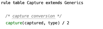
First, all the BaseLanguage types have corresponding dataforms, and in addition there are definitions of types that are only ever used during type checking, such as capture type.
The macros in Types macro table define the rules how types are constructed, ensuring, among other things, that bounds on type parameters are correctly processed.
(examples of type dataforms)
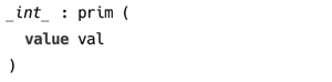
Primitive types define allowed ranges, so the dataforms for these types have value slots capturing literal’s value.
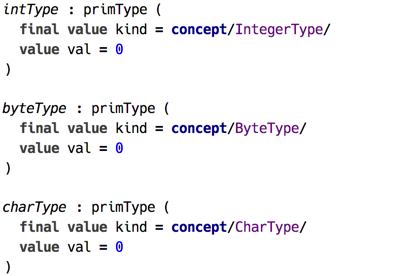
(examples of primitive type dataforms)
There are two queries defined for type checking and for converting a type to another type. The latter is used when testing for subtyping. ConvertsTo query expands both its parameters before activating convertsTo() constraint, which launches the processing of the relation.
(the production from ConvertsTo query)
(the production from Typecheck query)
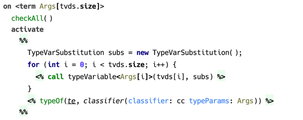
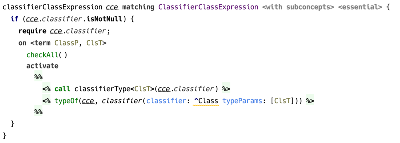
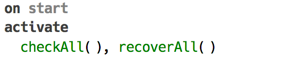
Typechecking itself starts with activating the checkAll() constraint, triggering the productions responsible for assigning types to literals, this expression, as well as processing type annotations — ensuring that these are built without violating bounds.
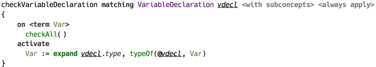
The rule for variable declaration is quite trivial: the type annotation gets expanded to dataform and assigned to the source location with typeOf() constraint.
(assigning the type to a variable declaration)
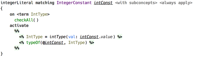
An integer literal is simply assigned the type int with the value being the value of literal.
(assigning the type to int literal)
From these starting points type checking continues up the syntax tree until there are no more productions left that can be triggered.
A dot expression propagates the type from operation to the whole expression.
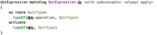
(typechecking of dot expression)
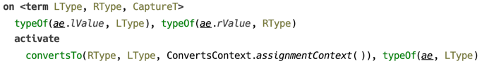
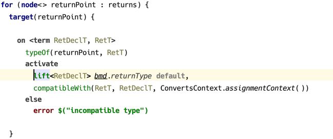
Whereas assignment does something more: it ensures that the actual type on the right is compatible with the type on the left.
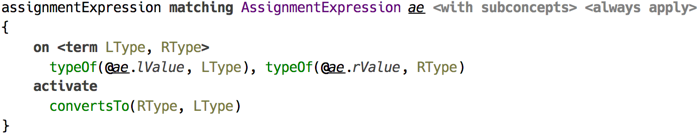
(typechecking of assignment expression)
Type Relations
Several kinds of relations on types are defined, surveyed in the following table.
| Relation | Constraint | Description |
|---|---|---|
| compatibility | compatibleWith() |
generalisation of conversion to include void type |
| conversion | convertsTo() |
generalisation of subtyping, LSP |
| primitive subtyping | primSubtype() |
subtyping among primitive types |
| subclassing | promote() |
subtyping among classifier types |
| containment | containedIn() |
type parameter containment |
Conversion
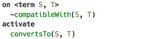
Constraint convertsTo() ensures that a type can be converted to another type, that is a type A can be used instead of type B. To test if a type is acceptable in certain locations, including those that allow any type, the constraint compatibleWith() is used, which delegates to convertsTo().
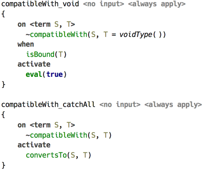
(resolution of compatibleWith() via convertsTo())
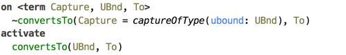
In its turn, convertsTo() delegates to either primSubtype(), which is responsible for solving primitive subtyping, or to promote(), which focuses on subtyping of classifier types.
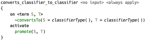
(convertsTo() delegates to promote() for classifier type)
Subclassing
Resolution of promote() constraint, which represents subtyping among classifier types, is implemented around a simple idea of representing all subclass paths the root (Object) to a classifier as a set of lists. This representation deliberately ignores the class parameters. As a first step, the shortest path from supertype’s classifier to subtype’s one is selected. This path is then reversed and represented as a dataform list. This makes it possible to pattern-match on this list, since it is nothing more than a cons list represented as a dataform.
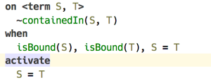
Subtyping is a reflexive and transitive relation, so promote() is replaced with another constraint dpromote(), which triggers one of the two productions responsible for either aspect of the relation. Transitivity is solved by advancing up the supertype path keeping track of all type variables and ensuring all bounds on type parameter are satisfied. Reflexivity delegates to containedIn() to ensure parameters are within bounds, which in its turn delegates to convertsTo().
Take a simple example of Long classifier type — the boxed long. Its superclasses are written as follows.
  Long : Comparable : Object
  Long : Number : Serializable : Object
Suppose we need to decide if Long <: Serializable, that is if Long is a subtype of Serializable. The shortest path between those consists of three nodes : [Long, Number, Serializable]. Constraint dpromote() is activated with this list as the 3rd parameter, and it requires two steps of inductive production and one step of reflexive to solve this relation.
Typechecking Extended STLC
Simply Typed Lambda Calculus (STLC) is a famous example favored by textbook authors. This sample demonstrates how a classical type checking algorithm (Hindley-Milner1) designed for this language can be implemented using Coderules. It also presents two substantial extensions to basic Hindley-Milner type inference: type annotations and typeclasses from Haskell. They will be discussed in succession, highlighting some of the useful features of Coderules language and implementation challenges that typesystem itself introduces. These extensions show that even an advanced typesystem can be implemented using Coderules, and in a natural way rule-based way.
For purposes of keeping this sample a bit simpler, we keep the language confined to boolean values. Aside of boolean constants True and False, the mandatory lambda abstraction and application, let-in expression, and if-then-else, we have in addition defined pairs of values and fix operator to support recursion.
The syntax of presented lambda calculus is compatible with Haskell, and consequently all examples can be typechecked with, for example, GHC (Glasgow Haskell Compiler). The required extensions for GHC are:
- for basic STLC:
UnicodeSyntaxandExplicitForAll; - for STLC with type annotations: additionally,
ScopedTypeVariablesandRankNTypes; - for STLC with typeclasses: additionally,
FlexibleInstances.
The dataform table is trivial, there’re two terms used in Cons-list implementation (Cons and Nil), term Constraint used in the part of typesystem concerned with typeclasses, and other expected terms for types (Fun for function type, Forall for universal types etc.).
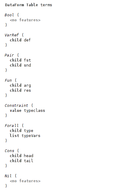
(dataform table)
There is only one query of kind TYPECHECK, which launches types recovery. All the type checking is done by the automatic productions “on start”.
Basic Hindley-Milner Type Inference
The basic type inference is covered by the several handlers: handler typeOf that contains most of the typing rules, handler forall covers typing of universal types, recover handler is concerned with translating inferred types back to SNodes representation, and consList is an utility handler.
Cons-list
Handler consList is a straightforward implementation of Cons-list, present in all functional programming languages. Implementation consists of Cons and Nil data forms, append constraint and two rules that process it, one for common case and one for base case (when one of the input lists is empty).
There’s also a helper function, that translates lists embedded in Coderules to these ad-hoc Cons-lists.
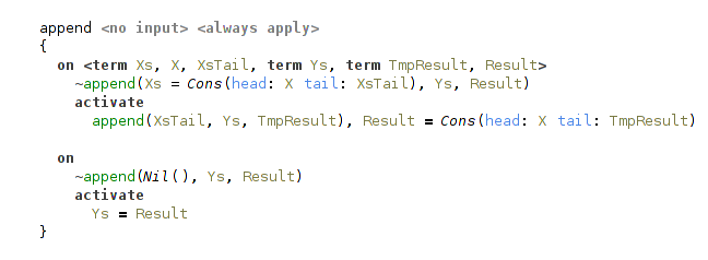
(single rule implementing cons-list)
Main Typechecking Rules
Handler typeOf contains most of the type inference rules.
Besides typeOf constraint it also declares a helper constraint newTypeVars.
Its role is simple, it collects newly introduced type variables.
It is needed for later generalization on let-bindings.
Type variables are introduced at lambda-bindings and at instantiations of universal types.
Fresh type variables are represented simply by fresh logical variables.
For example, this is a rule for lambda-bindings:
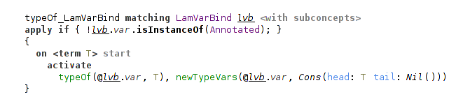
(typing rule for a lambda-binding)
It’s important to note that these variables can later be bound to something during the process of type inference, and so just before generalization on let we need to additionally check that the variables are indeed free.
Actually, the process of collecting free type variables could be implemented on the language level with a something like a predicate term_variables/2 from Prolog, instead of manual tracking using newTypeVars constraint.
Typing rules for the most of the nodes are straightforward: rules match on typeOf and newTypeVars constraints of the node’s children and produce these in their turn.
There’re additional conditions on some of the rules, because their handling depends on whether these nodes are annotated or not. The case with annotations is processed in another handler annotation.
For example, in the case of unannotated let-binding we simply generalize over all free variables in the bound expression:
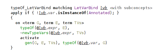
(typing rule for a let-binding)
In the typing rule for variable occurrences they are instantiated with a help of inst constraint.
It also returns a list of fresh instantiated variables.
This rule ensures that terms with universal types can actually be used polymorphically.
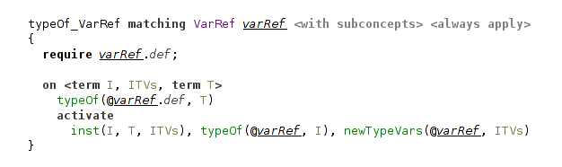
(typing rule for a variable reference)
The type checking for if-then-else ensures that the types of both branches unify, and assigns the resulting unified type to the whole expression.
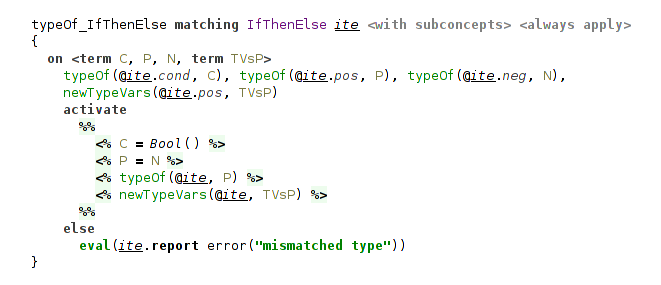
(typing rule for conditional expression)
The most interesting rule here is for function application. Besides instantiating function, which may has polymorphic type, it also checks that the function can be applied to the argument, according to the types.
The subsumption relation on types, that checks this, comes from the need to account for type annotations and is covered later. In short, it handles the case when the actual argument has a more general (more polymorphic) type, than type of the formal parameter. In other words, when the parameter’s type is subsumed by the argument’s type. In the basic STLC formulation we would have here a usual unification between parameter’s type and actual argument’s type.
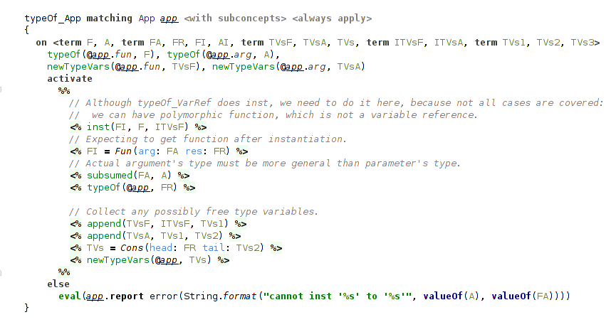
(typing rule for function application)
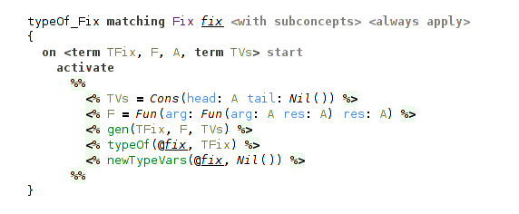
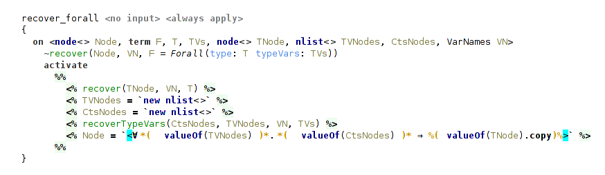
Finally, the fix operator, which represents general recursion, is given the type ∀a. (a → a) → a.
(typing rule for fix operator)
Typechecking Universal Types
A separate handler is dedicated to producing and instantiating universal types, and it is the most interesting part of STLC.
The handler declares two general constraints gen and inst together with several helper constraints.
Generalization
gen constraint returns universal type through the logical variable passed as the first argument, accepts the type to generalize in the second argument and the type variables to generalize over (collected with newTypeVars constraint) in the third.
gen activates 2 helper constraints: the first processes type vars one by one (that’s where the main work happens), and the second handles several different cases depending on the form of type that is generalized.
(rule for a type generalization)
Generalization of a single free type variable consists from two steps.
The first step is concerned with typeclass constraints on type variables, and will be explained in the corresponding section below.
In short, we need to get the type constraints, that the type variable collected during type inference, and fix them, because they become a part of the definition of type variable in its type scheme and mustn’t change.
The second step is a substitution of its occurrences in the generalized type with references to a fresh type variable playing a role of its definition.
This is accomplished simply by a unification of free type var with VarRef data form, pointing to this fresh type var.
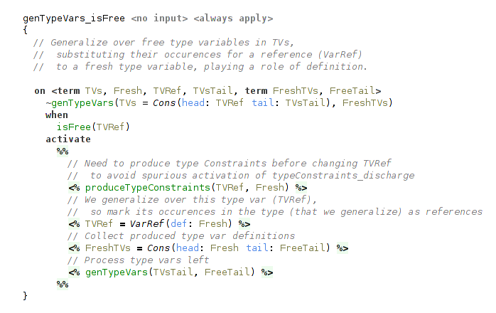
(generalization of a single type variable)
The fresh type variables are collected and then passed to the second helper constraint, that actually produces universal type. It may appear, that in the type there’re no free type variables to generalize over. In this case we shouldn’t produce universal type.
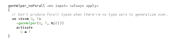
(not generalizing with no free type variables)
In another case, when the generalized type is itself a universal type we merge the sets of the generalized type variables to avoid nested universal types.
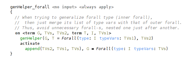
(generalization of a universal type)
And in the common case we just produce a universal type with processed type variables.
(generalization, common case)
For example, generalizing a type Fun(arg: A res: B), where A and B are free terms (type variables) we will get Forall(type: Fun(arg: VarRef(def: C) res: VarRef(def: D)) typeVars: [C, D]), where C and D are fresh variables.
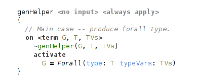
Instantiation
Instantiation of a universal type mirrors generalization of a type.
inst constraint also depends on the form of a type being instantiated.
There’re two cases: the trivial case, when the instantiated type is not a universal type, and the common case, when the instantiated type is really a universal type.
In the former case we essentially do nothing, and return the same type and an empty list of instantiated type variables.
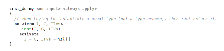
(instantiating non-universal type)
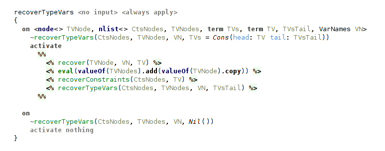
The latter case uses a helper constraint, that processes bound type variables from universal type one by one.
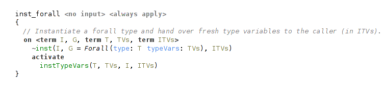
(instantiating universal type)
Instantiation of a single bound type variable has two steps.
The first step is a substitution of all references to bound type variable with a fresh term.
It is done with a call to subst, a part of the internal API.
The second step is concerned with typeclass constraints. What we need to do here is to instantiate (copy, really) the set of typeclass constraints for the freshly instantiated type variable.
This variable is collected to the list of instantiated type variables for the caller.
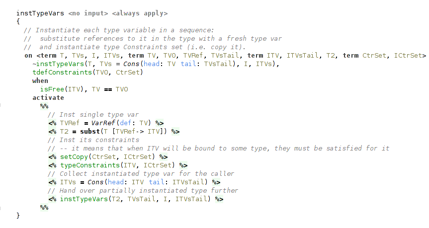
(instantiating single type variable)
Outputting Types
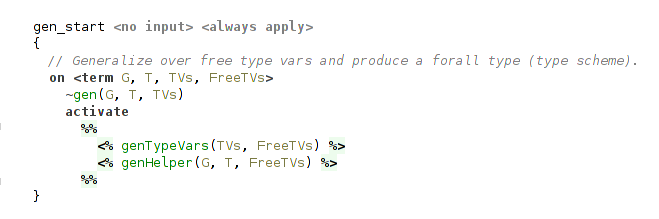
The handler recover is responsible for translating the calculated types to SNode form and is pretty straightforward. On each typeable node a recover constraint is activated. SNodes representing types are constructed using quotations.
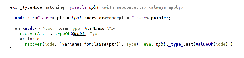
(starting type recovery)
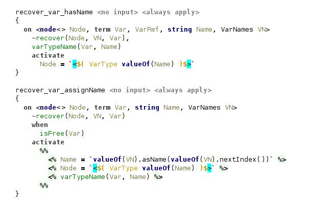
The rules for type variables ensure that every one of them has an assigned name.
For variables without names assigned in type annotations the second rule will assign them with a help of VarNames utility.
(recover type variable)
The most involved rule is for universal type, because it requires to recover and collect in a list SNodes representing type variables. Analogously, for each type variable we need to recover and collect its typeclass constraints.
(recover universal type)
(recover bound type variable from universal type)
Next, we turn our attention to the extensions to STLC.
Type Annotations
Extension of STLC with type annotations demonstrates two important points: a usage of Coderules macros and an implementation of a relation between types in the form of constraint. Relations on types are present in many typesystems, and probably the most widespread example is a subtyping relation (e.g. isSubtype(type1, type2)). As a matter of fact, the subsumed relation, presented here, is a form of subtyping too, as explained below.
Macros
Coderules macros can help to keep the formulation of a typesystem cleaner, by moving out to a macro table some routine tasks, such as creating complex terms or building dataform representations of SNodes. For such cases macros can be viewed as a form of constructors, when creation of a dataform requires, for example, recursive creation of subterms or production of constraints.
In this lambda calculus there’s a single macro table called types for translation of SNodes, representing type annotations, to corresponding dataforms for manipulation in Coderules program.
A typical example of a macro is for the function type. It recursively invokes macros for its argument and result types.
(macro for a function type)
Macro for a type variable produces a fresh logical variable each time it is invoked.
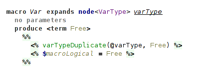
(macro for a type variable)
As it can be invoked several times, we need to unify different logical variables emitted for a single type variable.
It is done in handler annotation.
We also emit a special constraint to carry type variable’s name.
It’s needed for outputting types in handler recover with expected names.
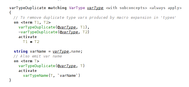
(unifying duplicate logical variables)
Typing Rules for Annotations
All these macros are used in the handler annotation in a rule that produces a single constraint carrying the type from annotation:
(usage of a macro expansion)
Handler annotation defines several important rules.
Two of them are concerned with special handling of annotated bindings (let-binding and lambda-binding).
For lambda-binding we simply propagate the type from annotation, because at this point, at the introduction of a new variable, there’re no constraints on it to check against.
(annotated lambda-binding just assigns to its variable type from the annotation)
The case of let-binding is different. Here we need to check the annotation against the inferred type of the bound expression. This is done with a help of subsumed constraint, explained below. It is the only difference of this typing rule from a rule for unannotated let-binding.
(annotated let-binding checks annotation against inferred type with subsumed)
Another rule is concerned with annotated expressions. In this case we check against the type of inferred expression, analogously to the rule for let-binding.
(annotated expression also includes subsumed check)
In essence, this is all that is special about type annotations.
Most of the work and complexity is about subsumed relation to make the typesystem more expressive: it is concerned with higher-rank types.
We can substitute all occurrences of subsumed constraint for the unification predicate and get a usual STLC with simple type annotations, that must be equivalent to inferred types everywhere.
The following discussion is mostly concerned with a description of aspects of the typesystem and less so with Coderules.
Higher-Rank Polymorphism
Type annotations provide us with a better understanding of the code. For example, in Haskell it is considered a good practice to write type annotations for all top-level definitions. But code documentation is not the only application of type annotations.
Hindley-Milner type inference is a very powerful typesystem and allows to write very generic programs without type annotations at all.
But that conciseness comes at a price. This typesystem doesn’t cover all terms that a programmer would like to write.
For example, this construct is not typeable within Hindley-Milner typesystem: let f = (\g → (g True, g 42)) in f (\x → x), but f here could have a type (∀a.a → a) → (Bool, Int).
You can also imagine a case, where you want to operate on heterogeneous lists with a polymorphic function: f (g :: (∀c. [c] → Int) = g ["hello"] + g [1,2]. Here f has a type f :: (∀c. [c] → Int) → Int.
And this is a perfectly sane case for functional programming!
There comes a notion of higher-rank polymorphism.
Hindley-Milner typesystem can only infer rank-1 types.
Rank-1 types have only a single outer-most universal quantifier.
For example, a familiar function map has a type map :: ∀a b. (a → b) → [a] → [b].
If a type contains quantifiers only to the right sides of arrows, it is a rank-1 type too.
It’s because inner quantifiers can be “floated out” to the outer level without a loss of generality.
So, such types are essentially equivalent to the types with a single outer-most quantifier.
For example, compare these types: ∀a b. a → b → a and ∀a. a → (∀b. b → a).
They behave in the same way in all possible uses.
Things become more interesting when we want to accept polymorphic types as arguments to functions.
Notice that these two types for a function f from a previous example mean something completely different:
f :: (∀c. [c] → Int) → Int and f :: ∀c. ([c] → Int) → Int.
With a second type f just wouldn’t typecheck.
That’s why we can’t “float out” quantifiers that appear as arguments to functions.
Such types are called higher-ranked types.
Formally, the rank of a type is how deep universal quantifiers are nested to the left side of arrows, that is, a number of these arrows.
For example, these are rank-2 types: (∀a. a → a) → Bool and (Bool → (∀a. a → a)) → Bool, while that is a rank-3 type: ((∀a. a → a) → Bool) → Bool.
Higher-ranked types can’t be inferred without a help from the programmer in the form of type annotations. Programmer can provide type annotations in the cases where he needs something more expressive. Actually, rank-2 types are sufficient for most of the use cases, but the machinery required for typing them contains all of the features needed for typing arbitrary higher-ranked types. This case, where programmer can make some types more general then they would be inferred, requires a noticeably more involved typesystem. Theoretical treatment of typesystems handling type annotations on top of Hindley-Milner type inference can be found in several papers, with a closest one to the current implementation in 2 (and this paper, probably, is more accessible).
For the implementation it means that we need to check that the type annotation provided for a term agrees with all its usages. Specifically, that the term (i.e. its type) can be instantiated to the type, required by its usage.
Subsumption Relation
Handler subsumption defines one main constraint subsumed that follows a dsk relation from the corresponding paper2.
subsumed implements a form of subtyping between polymorphic types, where less general type is a subtype of a more general (more polymorphic) type.
It means that if type A can be instantiated to type B, then type A is more general than type B.
This relation subsumed(B, A) can be read as: “type B is subsumed by type A” that means “type B is less polymorphic than type A”.
A minor note is that directions of subsumed and dsk relations are opposite, so where dsk(A, B) holds, there subsumed(B, A) holds.
Although dsk and subsumed behave in the same way, there’re some important differences between theoretical treatment of this relation and its implementation in Coderules.
Formal definition of a dsk needs to take into account some details, which in the case of subsumed are handled by Coderules.
For example, tracking variable names to avoid invalid cyclic substitutions (that is, to perform occurs check), that in Coderules is done during unification.
So Coderules can actually reduce the burden lying on a developer implementing a typesystem and trying to closely follow its theoretical treatment.
Subsumption proceeds by pattern matching on types in question. As we computing a relation between polymorphic (i.e. universal) types, the most important rules are concerned, of course, with universal quantifiers. There’re two cases for this, depending on which side of relation the universal type is. Before the check the universal types are instantiated (i.e. type variables in them are substituted for fresh logical variables). Then we proceed with recursive subsumption check on these instantiated types. The most important part comes after that: we need to check that the types, to which type variables are instantiated, are valid and consistent. The required checks differ for these two rules. That’s where the asymmetric nature of relation manifests itself. For details, the reader can proceed to an example for polymorphic pair types described below or, for a full treatment, to the original paper.2
(subsumption rules for universal types)
Another important case is that of leaves, when one of the types is either a type variable reference or a free type variable (either instantiated or initially free, that is, not bound during the process of type inference). In the case of free type variable we unify it with another term, essentially instantiating type variable to it. If there will be conflicting instantiations of the same type variable to different types, unification will fail and halt typechecking.
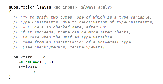
(leaves in subsumption are unified)
But if the second term is a free type variable too, then unification will succeed and we may need to perform additional check.
For example, consider checking subsumption relation for this case: ∀a b.(a,b) ≤ ∀c.(c,c).
As you can see, subsumption relation doesn’t hold here, because the second type is not more general than the first.
In the subsumption rules for universal types all bound type variables will be instantiated, and we will need to check subsumed(Pair(A,B), Pair(C,C)), where A, B and C are free (instantiated) type variables.
Rule for leaves will successfully unify A with C and then also B with C, and we will get A=B=C.
But this is certainly not what we want!
That’s why, besides unification in the rule for leaves, we need an additional check ensuring that there’re no conflicting instantiation of one type variable to several different type variables.
This check is relevant only for free type variables coming from the instantiation of universal types.
So it is performed only in the rules for universal types.
In the case of variable references (that is, type variables bound by some universal quantifier) they must match because these variables are rigid, and they can’t be unified. This case is essentially the same as in Haskell, where, for example, two type variables with different names entered by a user can’t be unified.
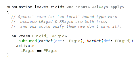
(rigid type variables in subsumption are checked for equality)
Subsumption rule for function types proceeds by checking argument and result types. It is analogous to typical subtyping rules for function types: argument types are checked contravariantly, result types are checked covariantly.
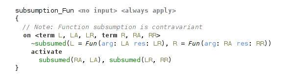
(subsumption rule for function type)
Rule for a pair type is straightforward.
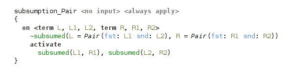
(subsumption rule for pair type)
That’s how implementation of a complex relation on types can look like in Coderules.
Typeclasses
Haskell typeclasses are one of the most important and complex features of its typesystem, that distinguishes Haskell among other well-known functional languages. Implementing typeclasees using Coderules shows that it has expressive power that is sufficient even for the advanced typesystems. This implementation partly relies on the reference Haskell typechecker3.
Note about notions: by the word “constraints” are meant Coderules constraints, whereas typeclass constraints are called in this qualified way (“typeclass constraints”), or with an uppercase letter (“Constraints”) to avoid ambiguity.
Typeclass Constraints
In essence, typeclasses extend typesystem by adding a kind of requirements, Constraints on type variables that are bound by universal quantifier. Typesystem needs to carefully track that universal types are instantiated only to the types satisfying their Constraints, and that the types are generalized to universal types properly, without leaving out any Constraints.
For example, we can instantiate a universal type ∀ a. (C1 a, C2 a) ⇒ (a, a) → a only to a type that satisfies both Constraints C1 and C2.
Or, in case of a generalization, given a function mappend ∷ ∀ a. Monoid a ⇒ a → a → a, for a function f in let f = (\x → mappend x x) we must infer a type ∀ t. Monoid t ⇒ t → t.
Everything else is mostly a matter of other language aspects (structure, editor and constraints aspects) and not of a typesystem. Still, it’s important to note, that typesystem doesn’t need to check that type variables are properly scoped, because it is handled by “constraints” language aspect. It slightly simplifies the typesystem.
So, existing typesystem needs to be modified only in the places concerned with universal types:
- modification of generalization & instantiation of type variables in
forallhandler; - straightforward additions in macro table
typesandrecoverhandler.
The major part of typechecking typeclasses is placed in several new handlers:
- handling declarations of typeclasses and its instances — in
typeclasseshandler; - processing typeclass constraints (collecting and checking them) — in
typeConstraintshandler; - implementation of the Set data structure, used mainly in
typeConstraintshandler — insethandler.
Now, let’s move through these handlers.
Set Data Structure
Handler set implements the Set data structure together with several utility functions.
A set is represented as a number of set constraints in the constraint store.
Each set constraint has 2 arguments: the first argument is a free logical variable representing handle for the data structure and the second argument is an element belonging to it.
As an example, a set {a, b, d} (where a, b and d are some dataforms or free logical variables) will be represented as three constraints: set(S1, a), set(S1, b) and set(S1, d), where S1 is a Set handle.
Programmer can manipulate the set with a handle.
The implementation consists of a single rule that maintains the set invariant, i.e. that it can’t contain two equal elements.
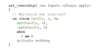
(set data structure implementation)
The beauty of such representation of a set is that merging sets comes essentially for free and, moreover, is performed implicitly. To merge two sets a programmer only needs to unify their handles. And there one crucial feature of Coderules enters the picture: constraint reactivation. When arguments of inactive constraints in the constraint store change (for example, are unified with something), these constraints are reactivated.
Consider the following example.
Assume there’re two sets S1 = {a, b} and S2 = {a, c} and the constraint store contains four constraints representing them: set(S1, a), set(S1, b), set(S2, a) and set(S2, c).
Next, unification of logical variables S1 and S2 happens (S1 = S2).
Due to automatic reactivation, all inactive constraints in the store that refer to these unified variables will be activated again.
Because of this they will be tested for matching on the rule maintaining set invariant.
In this particular case it will be triggered on the constraints set(S1, a) and set(S2, a) (remember, here S1=S2) and discard one of them.
After this constraint store will contain only three set constraints (set(S1, a), set(S1, b) and set(S1, c)), representing the result of merging {a, b} and {a, c}, a set {a, b, c}.
The implementation of a set is also an example of one useful Coderules pattern: maintaining some invariant assumed by other rules using a top-level rule, that will be matched first and ensure invariant.
Handler set also declares several utility functions with straightforward implementations:
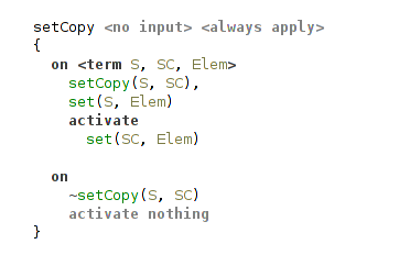
- copying a set;
- making a Cons-list out of a set while removing the original set;
- making a Cons-list out of a set while preserving the original set;
- testing whether one set is a subset of another.
(copy a set)
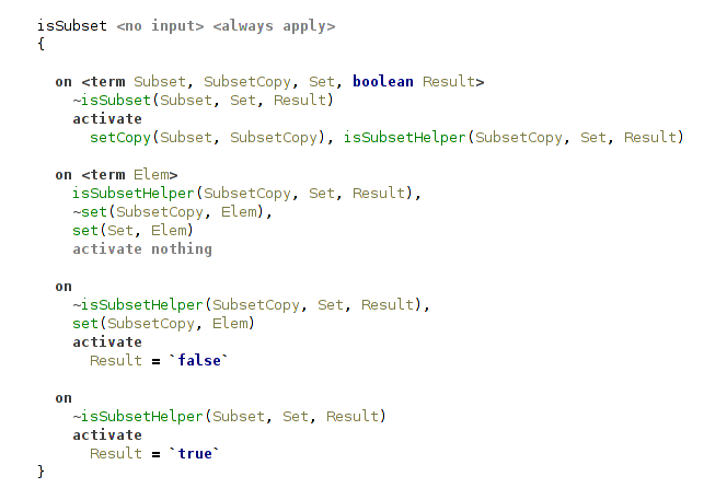
(test whether one set is a subset of another)
Representation of Typeclass Constraints
Typeclass constraints are used in 2 roles during type checking: in definitions of type variables bound by quantifiers and as requirements on types.
Handler typeConstraints declares 2 constraints that correspond to these 2 roles: tdefConstraints and typeConstraints.
They map a type variable to a set of its typeclass constraints.
Contrast it with how type variables are represented: they’re explicitly stored in a list in the Forall dataform.
Thus, typeclass constraints on a type variable are stored implicitly, not inside the Forall dataform, but in the constraint store.
Their representation as a set greatly simplifies working with them.
During the process of type inference free logical variables representing yet unknown types can be unified.
Previously we haven’t given much thought to it, unification just happened without our attention.
But now consider this question: what changes when free type variables can carry sets of typeclass constraints?
The answer is that we should merge these sets when variables are unified.
But at which point? The problem is that unification can happen at any point (in any rule) during type inference.
And that’s where constraint reactivation again helps us, now for typeConstraints and tdefConstraints.
The following rule is a top rule in handler typeConstraints.
It ensures, that each type variable has a single set of all its typeclass constraints.
.png)
(merging Constraints sets)
It is clear how to collect typeclass constraints during the process of type inference. But what we further need to do with this set of typeclass constraints depends on what happens to the type variable. There’re two cases: it either remains free until the point of generalization (i.e. let-binding) or it is bound to a type.
Checking Typeclass Constraints
When free type variable becomes bound to something, we need to check that all typeclass constraints collected up to this point are satisfied. Due to constraint reactivation, another rule that starts this check will be triggered.
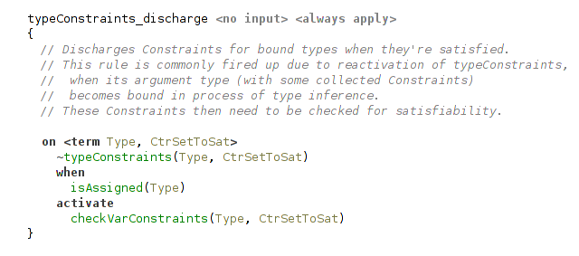
(rule playing a role of entry point to typeclass constraints check)
There’re 2 cases: it can be bound to a ground type (e.g. function type, Bool) or a type variable reference. The cases differ and require different checks.
(check collected typeclass constraints for a type variable: 2 cases)
Strength Check
First, let’s consider a slightly less obvious case of a type variable reference.
It refers to a type variable bound by some universal quantifier, and so, as part of its definition, has its own set of typeclass constraints.
This set must be more restrictive than the set of collected typeclass constraints we need to satisfy.
In other words, the type variable can’t be instantiated to a type (here, type variable reference) that doesn’t satisfy its typeclass constraints.
To check it we need to ensure that for each Constraint from the set of collected ones there’s a matching Constraint to satisfy it.
It can be done with a isSubset check.
(strength check: checking the restrictiveness of two Constraint sets)
For example, given a function application f x with types x ∷ C1 t ⇒ t (t is bound somewhere else) and f ∷ ∀ a.(C1 a, C2 a) ⇒ a → a, the strength check will clearly fail, because the Constraints set {C1} on the type variable t is not more restrictive than the set {C1, C2}. The set {C1, C2} is not a subset of {C1}.
Instance Check
The second case of a usual type is more intuitive and more common, but its implementation is a bit more involved. The first two rules in it do nothing special: the first makes a list out of the set and the second traverses it, triggering actual instance check for each typeclass constraint on a type.
.png)
(instance check, first two rules)
The next two rules try to find a matching instance among all instances of the typeclass with a help of instance constraint.
It is present in the constraint store for each declared typeclass instance in a program.
Typeclass instances can be declared not only for types but also for type schemes.
For example, Haskell has the following instance of Monoid typeclass: instance Monoid [a] where the instance is declared for a universal type forall a. [a]. Compare it to instance Monoid Bool where we have a usual type Bool.
That’s why we need to try instantiating the type scheme from instance declaration to the type in question.
It is done with a combination of inst constraint and unification.
It’s important to note, that instantiation here may trigger recursive instanceCheck.
For example, consider how instanceCheck(Pair(Bool, Bool), {Monoid}) proceeds in presence of instance Monoid Bool and instance (Monoid a, Monoid b) => Monoid (a, b) in a program.
Here we first need to find an instance for pairs, and then additionally check its own Constraints: that there exist instances for both element types of a pair. The type (Bool, Bool) satisfies this requirement given these 2 instances.
The last rule simply fails in case when no matching instance is found.
The typecheck is failed by triggering eval(false).
Of course, it isn’t the best mechanism for reporting typesystem errors, but it’s a temporary solution.
.png)
(instance check: searching for a typeclass instance for a type)
Universal Types and Typeclass Constraints
Typeclasses require only a little change to forall handler.
In the rule for generalization of a type variable we have to add only a single production that moves collected typeclass constraints (in typeConstraints) to a definition (tdefConstraints).
(generalization over a single type variable: notice activation of produceTypeConstraints)
(collected typeclass constraints become part of the type variable definition)
The constraint tdefConstraints is used in an instantiation of a type variable.
We essentially do the opposite: we copy typeclass constraints from the definition (tdefConstraints) to a new set (in typeConstraints) for a freshly instantiated type variable.
(instantiation of a single type variable: notice activation of typeConstraints with a copied set)
Typeclass and Instance Declarations
Handler typeclasses extends annotation handler and declares no new constraints.
It ensures the well-formedness of typeclass and instance declarations, and defines typechecking dependencies using require statements.
The rule for typeclass declaration only processes declaration of type variable declared in a typeclass and produces an auxiliary constraint carrying typeclass name, used in recover handler.
(processing typeclass declaration)
The rule for instance declaration is also straightforward. It expands a macro for its type scheme and produces instance constraint that is used in instanceCheck.
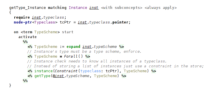
(processing instance declaration)
Typeclass contains a number of function Prototype declarations (i.e. pairs of symbol and type). The rule for them just produces their type given type annotation.
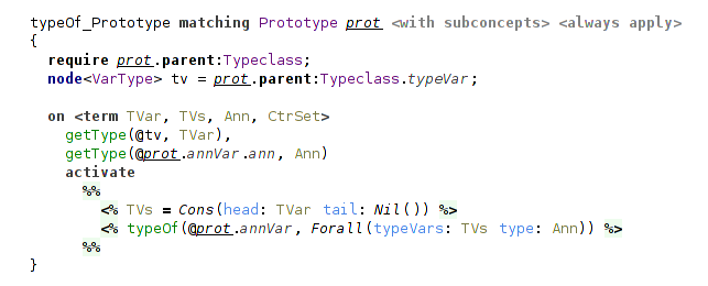
(producing type of a Prototype in a typeclass)
Instance, correspondingly, contains Prototype implementations, and they require the most involved rule. It checks that the actual type of the implementation agrees with a Prototype’s type. The first step of this is to instantiate the generic Prototype to the Instance type scheme. The second step is to actually check that the types agree, that is, the type of the implementation does not restrict the Prototype’s type (in other words, it is more general). It is checked using subsumption relation.
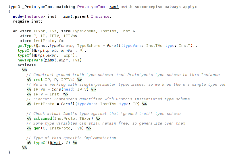
(checking correctness of Prototype implementations)
That is everything there is to the typechecking of typeclasses. To recap, the most important rules are concerned with processing typeclass constraints. They’re implemented in a way to be triggered automatically, while other rules heavily rely on this automatic and implicit checking of typeclass constraints.
-
See for example: Cardelli, Luca. “Basic polymorphic typechecking.” Science of computer programming 8.2 (1987): 147-172. ↩
Fitch Proof Validation
This example demonstrates the use of CodeRules to implement validation of logical proofs written using Fitch system. The idea of this implementation originates in the proof checking tool provided as part of an inroductory course on logic by Stanford University1. This overview serves for quick introduction, and more detailed information can be found at project’s home page (see the link on top of this page).
The four languages in this example define the structure of proofs (samples.fitch), the structure of three kinds of logic: Propositional logic, Herbrand logic, and First Order logic (samples.fitch.*logic).
The proof structure allows for building hierarchical proof trees, which are necessary for Implication Introduction rule, and interprets the leafs as reasonings, which can be either assumptions or judgements. The beginning of the proof contains all the premises, and the final top-level node is the goal.
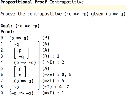
(example of proof in Fitch system)
Base inference rules are defined by samples.fitch.propositionalLogic language, with two other extending the set of rules appropriately. Herbrand logic extends this language with relations, functions, and quantifiers, whereas First Order logic adds equality. Each of the logics also define their own root proof concept.
The proof validation is done through type checking with the only type being “Ok”. There is one query of kind TYPECHECKING, which simply activates checkAll(). Every logical formula from reasonings is translated into a dataform, with logical variables taking place of quantifier variables.
Each reasoning has a conclusion, which is expanded to term and assigned to the source location with conclusion() constraint. In addition, at the start, all proof’s premises are marked as valid using valid(). The process then continues recursively, with every inference rule constructed according to a single pattern:
- the head ensures the conclusions of all rule’s bases (input premises) match the required form,
- the rule’s conclusion matches the required form, and
- all the bases are valid.
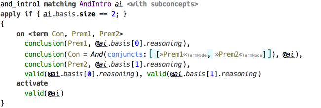
(example of an inference rule)
The rule’s body activates valid() constraint, therefore only reasonings that have met the requirement are marked as valid. Check handler marks reasonings that weren’t validated as erroneous.
Finally, if the proof’s goal is marked valid, it is assigned “Ok” type, otherwise it is marked with error.
-
Stanford Introduction to Logic http://logic.stanford.edu/intrologic/homepage/index.html ↩